第 10 章 WGCNA
10.2 默认参数(可选)
options(stringsAsFactors = FALSE)
# 打开多线程
enableWGCNAThreads()

# 官方推荐 "signed" 或 "signed hybrid"
# 用signed获得的模块包含的基因会少
type = "unsigned"

# 相关性计算
# 官方推荐 biweight mid-correlation & bicor
# corType: pearson or bicor
corType = "bicor"

corFnc = ifelse(corType=="pearson", cor, bicor)
# 对二元变量,如样本性状信息计算相关性时,
# 或基因表达严重依赖于疾病状态时,需设置下面参数
maxPOutliers = ifelse(corType=="pearson",1,0.05)

# 关联样品性状的二元变量时,设置
robustY = ifelse(corType=="pearson",T,F)
网络类型 (type):
“unsigned”:在无符号网络中,正相关和负相关被同等对待,这意味着基因可以被分到同一个模块中,无论它们是正相关还是负相关。这通常会导致模块更大,因为限制较少。“signed” 或 “signed hybrid”:有符号网络区分正相关和负相关。模块通常包含正相关的基因,导致模块更小且更同质化。注释正确指出,有符号网络通常会产生包含较少基因的模块。
相关性类型 (corType):
“pearson”:皮尔逊相关性测量变量之间的线性关系。它假设数据呈正态分布,对异常值敏感。
“bicor”:双权中值相关性(bicor)是一种稳健的相关性测量方法,与皮尔逊相关性相比,对异常值不太敏感。它在生物数据中非常有用,因为异常值较为常见。注释正确指出,“bicor”在生物数据中推荐使用,因为它的稳健性。
相关性函数 (corFnc):
使用 ifelse 根据 corType 选择相关性函数。对于皮尔逊选择 cor,对于双权中值相关性选择 bicor。
maxPOutliers:
这个参数在使用双权中值相关性时很重要。它设置可以被视为异常值的样本最大比例。对于皮尔逊相关性,这个值设为1,意味着不将任何样本视为异常值。对于bicor,典型设置可能是0.05,允许一些样本被视为异常值以提高稳健性。注释正确描述了这个参数的用途。
robustY:
这个参数在将基因表达数据与二元性状(例如疾病状态)相关联时使用。它决定是否在计算涉及二元变量的相关性时使用稳健方法。对于皮尔逊相关性,通常设为 TRUE,而对于 bicor,由于 bicor 本身是稳健的,所以设为 FALSE。注释准确反映了这个参数的用途。
# 导入分组信息
design <- fread("DATA/WGCNA/design.csv") %>%
  mutate(group = factor(group, levels = c("s_MiaFRFP",
                                          "s_Part1Lag",
                                          "s_Part1Lead",
                                          "s_Part2Lead",
                                          "s_Part3Lead",
                                          "s_Part4Lead")))
head(design)[1:2, 1:2]
##            run     group
##         <char>    <fctr>
## 1: SRR19913146 s_MiaFRFP
## 2: SRR19913145 s_MiaFRFP

traitData <- design %>%
  dplyr::select(sample, group) %>%
  dcast(sample ~ group, fun.aggregate = length, value.var = "group") %>%
  column_to_rownames("sample")
head(traitData)[1:4, 1:4]
##              s_MiaFRFP s_Part1Lag s_Part1Lead s_Part2Lead
## s_MiaFRFP_1          1          0           0           0
## s_MiaFRFP_2          1          0           0           0
## s_MiaFRFP_3          1          0           0           0
## s_Part1Lag_1         0          1           0           0

group_list <- design$group
# 导入 counts 数据
counts <- fread("DATA/WGCNA/counts.csv") %>%
distinct(name, .keep_all = T) %>%
dplyr::select(name, design$sample, everything())
head(counts)
## name s_MiaFRFP_1 s_MiaFRFP_2 s_MiaFRFP_3 s_Part1Lag_1
## <char> <int> <int> <int> <int>
## 1: ENSG00000228037 2 0 0 2
## 2: ENSG00000142611 2088 1753 2396 358
## 3: ENSG00000284616 0 0 0 0
## 4: ENSG00000157911 5039 3794 4870 2294
## 5: ENSG00000260972 0 0 0 0
## 6: ENSG00000224340 0 0 1 1
## s_Part1Lag_2 s_Part1Lag_3 s_Part1Lead_1 s_Part1Lead_2 s_Part1Lead_3
## <int> <int> <int> <int> <int>
## 1: 9 0 0 2 0
## 2: 272 264 204 228 328
## 3: 0 2 0 0 0
## 4: 1996 2352 2543 1666 2373
## 5: 0 0 0 0 0
## 6: 0 2 2 0 1
## s_Part2Lead_1 s_Part2Lead_2 s_Part2Lead_3 s_Part3Lead_1 s_Part3Lead_2
## <int> <int> <int> <int> <int>
## 1: 0 2 0 0 0
## 2: 225 136 235 210 331
## 3: 0 0 0 0 0
## 4: 2931 2624 3086 1928 2971
## 5: 0 0 0 0 0
## 6: 0 0 0 0 0
## s_Part3Lead_3 s_Part4Lead_1 s_Part4Lead_2 s_Part4Lead_3 gene
## <int> <int> <int> <int> <char>
## 1: 0 0 0 0 ENSG00000228037
## 2: 444 230 120 192 PRDM16
## 3: 0 0 0 0 ENSG00000284616
## 4: 3031 2048 2407 4193 PEX10
## 5: 0 0 0 0 ENSG00000260972
## 6: 0 0 0 0 RPL21P21
# 过滤低表达基因
mat <- dplyr::select(counts, design$sample)
rownames(mat) <- counts$name
# 筛选出至少在两个样本中表达的基因
keep_feature <- rowSums (mat > 1) >= 2 ;table(keep_feature)
## keep_feature
## FALSE TRUE
## 27268 35872
ensembl_matrix <- mat[keep_feature, ]
rownames(ensembl_matrix) <- rownames(mat)[keep_feature]
ensembl_matrix <- rownames_to_column(ensembl_matrix, var = "name")
library(biomaRt)
# 连接ensembl数据库
ensembl <- useMart("ensembl", dataset = "hsapiens_gene_ensembl")
# atr <- listAttributes(ensembl) # 查看数据库中有哪些信息
# 获得数据库中关注的 ID 信息
ids <- getBM(attributes = c("ensembl_gene_id", "hgnc_symbol","entrezgene_id"),
mart = ensembl)
# 修改列名
colnames(ids) <- c("ENSEMBL", "SYMBOL", "ENTREZ")
# 去除重复 ID
ids=ids[!duplicated(ids$ENSEMBL),]
# 连接基因 counts 矩阵和 ID 信息
All_gene_counts <- merge(ensembl_matrix, ids, by.x = "name", by.y = "ENSEMBL", all.x = TRUE) %>%
dplyr::select(name, SYMBOL, ENTREZ, everything())
# 以 SYMBOL 为行名的矩阵
symbol_matrix <- All_gene_counts %>%
dplyr::filter(!is.na(SYMBOL)) %>%
distinct(SYMBOL, .keep_all = T) %>%
column_to_rownames("SYMBOL") %>%
dplyr::select(design$sample)
dataExpr <- as.data.frame(lapply(symbol_matrix, function(x) as.numeric(as.character(x))))
rownames(dataExpr) <- rownames(symbol_matrix)10.3 表达量聚类分析
10.3.1 选择合适基因集,过滤缺失值
# 筛选关注的基因,并转换为行为基因名,列为样本名的矩阵。
## 策略 1:mad最大的前5000,
### 或者保留基因总数的前1/4(round(0.25*nrow(dataExpr)))。
### mad可以改为var(方差)。
### 如果要保留所有的基因进行筛选分析保留datExpr0 = t(dataExpr)。
dataExpr = t(dataExpr[order(apply(dataExpr, 1, mad), decreasing = T)[1:2000],])
dataExpr[1:4,1:4]
##              FAM83A    DPPA3     MMP1 HHLA2
## s_MiaFRFP_1       0 0.000000 9.189825     0
## s_MiaFRFP_2       0 0.000000 8.857981     0
## s_MiaFRFP_3       0 0.000000 7.636625     0
## s_Part1Lag_1      0 9.353147 4.807355     0
## 策略 2: 筛选中位绝对偏差前75%的基因,至少MAD大于0.01
# m.mad <- apply(dataExpr,1,mad)
# dataExprVar <- dataExpr[which(m.mad >
#                  max(quantile(m.mad, probs=seq(0, 1, 0.25))[2],0.01)),]
# dataExpr <- as.data.frame(t(dataExprVar))

# 检测缺失值
gsg = goodSamplesGenes(dataExpr, verbose = 3)
##  Flagging genes and samples with too many missing values...
##   ..step 1
if (!gsg$allOK){
  # Optionally, print the gene and sample names that were removed:
  if (sum(!gsg$goodGenes)>0)
    printFlush(paste("Removing genes:",
                     paste(names(dataExpr)[!gsg$goodGenes], collapse = ",")));
  if (sum(!gsg$goodSamples)>0)
    printFlush(paste("Removing samples:",
                     paste(rownames(dataExpr)[!gsg$goodSamples], collapse = ",")));
  # Remove the offending genes and samples from the data:
  dataExpr = dataExpr[gsg$goodSamples, gsg$goodGenes]
}

nGenes = ncol(dataExpr)
nSamples = nrow(dataExpr)
dim(dataExpr)
## [1]   18 2000
head(dataExpr)[,1:4]
##                FAM83A    DPPA3     MMP1 HHLA2
## s_MiaFRFP_1  0.000000 0.000000 9.189825     0
## s_MiaFRFP_2  0.000000 0.000000 8.857981     0
## s_MiaFRFP_3  0.000000 0.000000 7.636625     0
## s_Part1Lag_1 0.000000 9.353147 4.807355     0
## s_Part1Lag_2 1.000000 8.519636 3.584963     0
## s_Part1Lag_3 5.930737 4.954196 0.000000     0
10.3.2 样本层级聚类,查看有无离群值
sampleTree = hclust(dist(dataExpr), method = "average")
par(cex = 0.6)
par(mar = c(0,4,2,0))
plot(sampleTree, main = "Sample clustering to detect outliers", sub="", xlab="")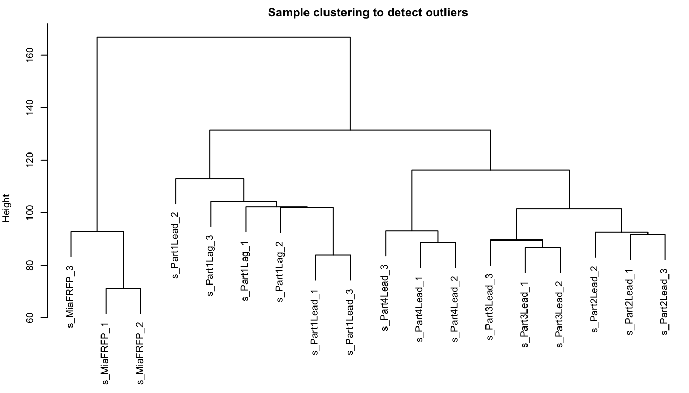
10.3.3 检查表型信息
datTraits = traitData
sampleTree2 = hclust(dist(datExpr), method = "average")
# 用颜色表示表型在各个样本的表现: 白色表示低,红色为高,灰色为缺失
traitColors = numbers2colors(datTraits, signed = FALSE)
# 把样本聚类和表型绘制在一起
plotDendroAndColors(sampleTree2, traitColors,
                    groupLabels = names(datTraits),
                    main = "Sample dendrogram and trait heatmap")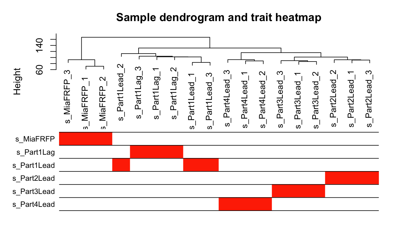
10.3.4 软阈值筛选
powers = c(1:10, seq(from = 12, to=30, by=2))
sft = pickSoftThreshold(datExpr, powerVector = powers, verbose = 5)
## pickSoftThreshold: will use block size 2000.
##  pickSoftThreshold: calculating connectivity for given powers...
##    ..working on genes 1 through 2000 of 2000
##    Power SFT.R.sq  slope truncated.R.sq mean.k. median.k. max.k.
## 1      1   0.0178  0.298          0.941 557.000  560.0000  842.0
## 2      2   0.2430 -0.602          0.942 233.000  225.0000  471.0
## 3      3   0.6520 -0.892          0.958 119.000  107.0000  301.0
## 4      4   0.8490 -0.984          0.977  68.500   55.8000  209.0
## 5      5   0.8910 -1.110          0.959  42.900   31.3000  157.0
## 6      6   0.9370 -1.150          0.981  28.700   18.4000  122.0
## 7      7   0.9550 -1.170          0.979  20.100   11.2000   98.6
## 8      8   0.9750 -1.180          0.989  14.700    7.1500   81.2
## 9      9   0.9780 -1.200          0.985  11.000    4.6900   68.4
## 10    10   0.9820 -1.210          0.988   8.520    3.1300   59.2
## 11    12   0.9630 -1.250          0.971   5.410    1.4800   46.3
## 12    14   0.9580 -1.260          0.974   3.660    0.7390   37.8
## 13    16   0.9430 -1.270          0.964   2.610    0.3920   31.8
## 14    18   0.9150 -1.300          0.950   1.930    0.2180   27.3
## 15    20   0.8520 -1.370          0.906   1.470    0.1280   23.9
## 16    22   0.8670 -1.350          0.927   1.150    0.0761   21.1
## 17    24   0.8720 -1.340          0.932   0.921    0.0466   18.9
## 18    26   0.8740 -1.360          0.930   0.750    0.0297   17.0
## 19    28   0.8910 -1.350          0.956   0.619    0.0191   15.5
## 20    30   0.9050 -1.350          0.959   0.518    0.0122   14.1
sft$powerEstimate #⭐推荐的软阈值
## [1] 5

## ⭐这个结果就是推荐的软阈值,拿到了可以直接用,无视下面的图。有的数据走到这一步会得到NA,也就是没得推荐。。。那就要看下面的图,选拐点。
## 根据我的经验,没有推荐软阈值,或者数字太大,后面跌跌撞撞走起来有些艰难哦,就得跑到前面重新调整表达矩阵里纳入的基因了。
## ⭐cex1一般设置为0.9,不太合适(就是大多数软阈值对应的纵坐标都达不到0.9)时,可以设置为0.8或者0.85。一般不能再低了。
cex1 = 0.9 #⭐👆
par(mfrow = c(1,2))
plot(sft$fitIndices[,1], -sign(sft$fitIndices[,3])*sft$fitIndices[,2],
     xlab="Soft Threshold (power)",
     ylab="Scale Free Topology Model Fit,signed R^2",type="n",
     main = paste("Scale independence")) +
text(sft$fitIndices[,1], -sign(sft$fitIndices[,3])*sft$fitIndices[,2],
     labels=powers,cex=cex1,col="red") +
abline(h=cex1,col="red")
## integer(0)
plot(sft$fitIndices[,1], sft$fitIndices[,5],
     xlab="Soft Threshold (power)",ylab="Mean Connectivity", type="n",
     main = paste("Mean connectivity")) +
text(sft$fitIndices[,1], sft$fitIndices[,5], labels=powers, cex=cex1,col="red")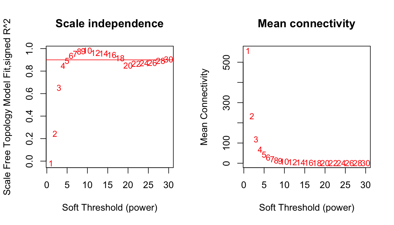
## integer(0)10.3.5 构建网络
如果前面没有得到推荐的软阈值,这里的power👇就要自己指定一个。根据上面的图,选择左图纵坐标第一个达到上面设置的cex1值的软阈值。
power = sft$powerEstimate
power
## [1] 5

net = blockwiseModules(datExpr, power = power,
                       TOMType = "unsigned",
                       minModuleSize = 30,
                       reassignThreshold = 0,
                       mergeCutHeight = 0.25,
                       deepSplit = 2 ,
                       numericLabels = TRUE,
                       pamRespectsDendro = FALSE,
                       saveTOMs = TRUE,
                       saveTOMFileBase = "TOM",
                       verbose = 3)
##  Calculating module eigengenes block-wise from all genes
##    Flagging genes and samples with too many missing values...
##     ..step 1
##  ..Working on block 1 .
##     TOM calculation: adjacency..
##     ..will use 7 parallel threads.
##      Fraction of slow calculations: 0.000000
##     ..connectivity..
##     ..matrix multiplication (system BLAS)..
##     ..normalization..
##     ..done.
##    ..saving TOM for block 1 into file TOM-block.1.RData
##  ....clustering..
##  ....detecting modules..
##  ....calculating module eigengenes..
##  ....checking kME in modules..
##      ..removing 39 genes from module 1 because their KME is too low.
##      ..removing 44 genes from module 2 because their KME is too low.
##      ..removing 52 genes from module 3 because their KME is too low.
##      ..removing 13 genes from module 4 because their KME is too low.
##      ..removing 11 genes from module 6 because their KME is too low.
##      ..removing 3 genes from module 7 because their KME is too low.
##  ..merging modules that are too close..
##      mergeCloseModules: Merging modules whose distance is less than 0.25
##        Calculating new MEs...

## 此处展示得到了多少模块,每个模块里面有多少基因
table(net$colors)
##
##   0   1   2   3   4   5
## 162 731 667 279  98  63

mergedColors = labels2colors(net$colors)
plotDendroAndColors(net$dendrograms[[1]], mergedColors[net$blockGenes[[1]]],
                    "Module colors",
                    dendroLabels = FALSE, hang = 0.03,
                    addGuide = TRUE, guideHang = 0.05)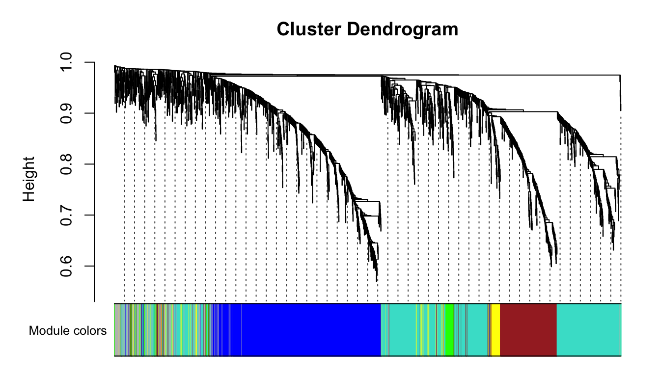
10.3.6 保存每个模块的基因
moduleLabels <- net$colors
moduleColors <- labels2colors(net$colors)
MEs <- net$MEs
geneTree <- net$dendrograms[[1]]
gm = data.frame(net$colors)
gm$color <- moduleColors
head(gm)
##        net.colors     color
## FAM83A          2      blue
## DPPA3           1 turquoise
## MMP1            3     brown
## HHLA2           2      blue
## OLFM4           5     green
## HSD3B1          1 turquoise
10.4 模块与表型的相关性
nGenes = ncol(datExpr)
nSamples = nrow(datExpr)
MEs0 = moduleEigengenes(datExpr, moduleColors)$eigengenes
MEs = orderMEs(MEs0)
moduleTraitCor = cor(MEs, datTraits, use = "p")
moduleTraitPvalue = corPvalueStudent(moduleTraitCor, nSamples)

#热图
# png(file = "6.labeledHeatmap.png", width = 2000, height = 2000,res = 300)
# 设置热图上的文字(两行数字:第一行是模块与各种表型的相关系数;
# 第二行是p值)
# signif 取有效数字
textMatrix = paste(signif(moduleTraitCor, 2), "\n(",
                   signif(moduleTraitPvalue, 1), ")", sep = "")
dim(textMatrix) = dim(moduleTraitCor)
par(mar = c(6, 8.5, 3, 3))
# 然后对moduleTraitCor画热图
labeledHeatmap(Matrix = moduleTraitCor,
               xLabels = names(datTraits),
               yLabels = names(MEs),
               ySymbols = names(MEs),
               colorLabels = FALSE,
               colors = blueWhiteRed (50),
               textMatrix = textMatrix,
               setStdMargins = FALSE,
               cex.text = 0.5,
               zlim = c(-1,1),
               main = paste("Module-trait relationships"))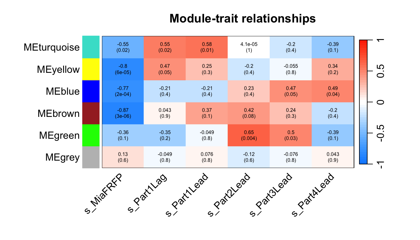
10.5 GS 与 MM
GS (Gene Significance) 定义:GS 是衡量单个基因与外部临床性状(如疾病状态、表型数据等)之间相关性的指标。 作用:通过计算每个基因的 GS 值,可以识别出与特定性状最相关的基因。这些基因可能在生物学上具有重要意义,因为它们与感兴趣的性状直接相关。 计算:通常是通过计算基因表达值与性状之间的相关系数来获得的。GS 值越高,基因与性状的相关性越强。 MM (Module Membership) 定义:MM 也称为基因模块成员关系,是衡量一个基因与其所在模块的特征向量(即模块特征基因,Module Eigengene)的相关性。 作用:MM 值表示一个基因在多大程度上与其所在模块的整体表达模式一致。高 MM 值的基因被认为是该模块的核心基因,通常称为“hub genes”。 计算:通过计算基因表达值与模块特征向量之间的相关系数来获得。MM 值越高,基因与模块的表达趋势越一致。
GS 关注的是基因与外部性状的直接相关性,帮助识别与特定性状相关的关键基因。 MM 关注的是基因与其所在模块的内部一致性,帮助识别模块中的核心基因。
modNames = substring(names(MEs), 3)
geneModuleMembership = as.data.frame(cor(datExpr, MEs, use = "p"))
MMPvalue = as.data.frame(corPvalueStudent(as.matrix(geneModuleMembership), nSamples))
names(geneModuleMembership) = paste("MM", modNames, sep="")
names(MMPvalue) = paste("p.MM", modNames, sep="")

# ⭐第几列的表型是最关心的,下面的i就设置为几。
# ⭐与关心的表型相关性最高的模块赋值给下面的module。
i = 2 #⭐
#module = "pink"
module = "turquoise"#⭐
assign(colnames(traitData)[i],traitData[i])
instrait = eval(parse(text = colnames(traitData)[i]))
geneTraitSignificance = as.data.frame(cor(datExpr, instrait, use = "p"))
GSPvalue = as.data.frame(corPvalueStudent(as.matrix(geneTraitSignificance), nSamples))
names(geneTraitSignificance) = paste("GS.", names(instrait), sep="")
names(GSPvalue) = paste("p.GS.", names(instrait), sep="")

column = match(module, modNames) #找到目标模块所在列
moduleGenes = moduleColors==module #找到模块基因所在行
par(mfrow = c(1,1))
verboseScatterplot(abs(geneModuleMembership[moduleGenes, column]),
                   abs(geneTraitSignificance[moduleGenes, 1]),
                   xlab = paste("Module Membership in", module, "module"),
                   ylab = "Gene significance",
                   main = paste("Module membership vs. gene significance\n"),
                   cex.main = 1.2, cex.lab = 1.2, cex.axis = 1.2, col = module)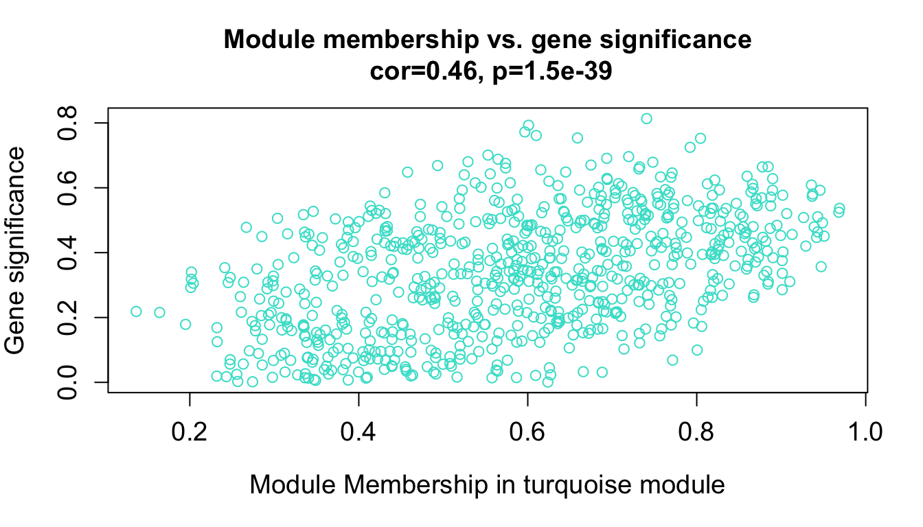
10.6 TOM
用基因相关性热图的方式展示加权网络,每行每列代表一个基因。 一般取400个基因画就够啦,拿全部基因去做电脑要烧起来了。 就想看看对角线附近红彤彤的小方块,以及同一个颜色基本都在一起,快乐。
nSelect = 400
set.seed(10)
dissTOM = 1-TOMsimilarityFromExpr(datExpr, power = 6)
## TOM calculation: adjacency..
## ..will use 7 parallel threads.
##  Fraction of slow calculations: 0.000000
## ..connectivity..
## ..matrix multiplication (system BLAS)..
## ..normalization..
## ..done.

select = sample(nGenes, size = nSelect)
selectTOM = dissTOM[select, select]
# 再计算基因之间的距离树(对于基因的子集,需要重新聚类)
selectTree = hclust(as.dist(selectTOM), method = "average")
selectColors = moduleColors[select]
library(gplots)
myheatcol = colorpanel(250,'red',"orange",'lemonchiffon')

plotDiss = selectTOM^7
diag(plotDiss) = NA #将对角线设成NA,在图形中显示为白色的点,更清晰显示趋势
TOMplot(plotDiss, selectTree, selectColors, col=myheatcol,main = "Network heatmap plot, selected genes")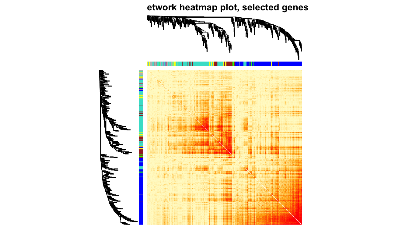
10.7 关注模块与表型的相关性
MEs = moduleEigengenes(datExpr, moduleColors)$eigengenes
MET = orderMEs(cbind(MEs, instrait))

par(cex = 0.9)
plotEigengeneNetworks(MET, "",
                      marDendro = c(0,9,1,2), marHeatmap = c(5,9,1,2),
                      cex.lab = 0.8,
                      xLabelsAngle = 90)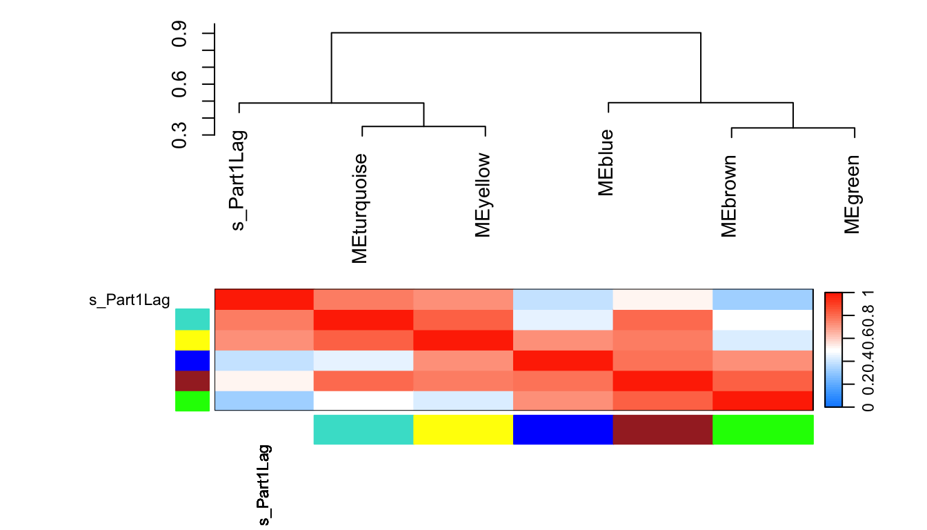
可参考教程: https://mp.weixin.qq.com/s/4N8eAStl0D7hL04G-4yICg https://www.youtube.com/watch?v=S7rFtZnA21o